
 |
 |
 |
 |
 |
 |
 |
 file:///C:/ENG_WEB/download.html
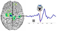
Inverse Solutions
Introduction and problem
statement: The discrete inverse problem
What about EEG/MEG source localization?: Two
Basic Principles
Methods that distort the source localization
estimates (how to select your
configuration)
What about LAURA?
What about ELECTRA?
Why using ELECTRA+LAURA?
What are the advantages of the irrotational
source model of ELECTRA?
A word of caution about ELECTRA: Misinterpretations of the irrotational model.
What about EPIFOCUS and ANA?
What is the p-value adjustment (correction) during
multiple test using EEG/MEG sources localization algorithms?
Robust methods for the analysis of EEG /MEG sources?
How we can evaluate the performance of source
localization algorithms?
What about LORETA sLORETA, etcetera ?
What about CarTool?
What about the WROP method?
The principle of shared autonomy and the evaluation of BCIs. Including videos showing that artificial intelligence alone can drive a wheelchair in a complex environment and even find its way out after entering a dead-end without any human intervention.
Comments on the document "Feature selection methods on Distributed Linear Inverse solutions for a Non invasive brain machine interface" by Laurent Uldry, Pierre W. Ferrez, Jose del R. Millan..
Inverse Solution
Introduction and problem statement: The discrete inverse problem
The so called inverse problem can be derived using the quasi static approximation of Maxwell equations. On these conditions the EEG/MEG measured at/near the scalp (v) is a linear function of the sources inside the 3D brain volume and the multiplicative factor is given by the lead field matrix (Neuroimage2004), that is,
(1) Lj=vA linear inverse solution of problem (1) also denoted linear source localization algorithm (SLA) can be represented by a matrix G that transforms back from the scalp to the brain volume to produce the estimated sources je:
(2) je=GvSubstituting (1) into (2) and (2) into (1) we obtain two fundamental equations for linear inverse problems:
(3) je=Rj where R=GL is the model resolution matrix and(4) ve=Dv where D=LG is the data resolution matrix.
The rows of the resolution matrix, denoted Resolution kernels describe the way simultaneously active sources affect the estimation of a single source.
The columns of the resolution matrix, denoted Impulse responses describe the way the inverse the inverse solution G estimate each single source alone.
Note that the general model is the model that considers sources in the whole 3D brain volume. Nevertheless, in some experimental situations, we can arrive to simpler models disregarding the contribution of some regions. For example:
-The cortical model is obtained by neglecting the contribution of sources far away from the surface of the cortex. Note that while the quadratic dependence with the inverse distance could justify the use of this model it has nothing to do with the believe that deep sources are not seen by the EEG or that deep structures form closed field configurations. Note that the necessary conditions for the latter (absolutely perfect symmetry of the source distribution and the anatomical structures) cast serious doubt about their existence in a real head, in addition, a negligible (under some a priori like grand averages of sensory data) magnitude is not a non existent (or null) magnitude.
-Dipolar models are obtained when the measured activity is supposed to be produced by a few regions of the brain.
- Single dipole model can be applied when the source of the measured data can be represented by a single dominant source. Note that there are efficient linear algorithms for the estimation of single dominant sources as EPIFOCUS (the first method with zero bias in dipole localization). In contrast to sLORETA that get distorted and need to be regularized for little noise in the data, EPIFOCUS localizes sources with minimal errors for clean or noisy data using a single inverse matrix.
On this page you will find information about the following inverse methods: LAURA, EPIFOCUS, ELECTRA, LORETA, sLORETA.
Back to TOPWhat about LAURA?
LAURA for Local Autoregressive Average is a regularization strategy inspired on the autoregressive models for spatial data proposed by Ripley mixed with the concept of averages and a pinch of biophysics. The main aspects of this implementation are:
L1) To facilitate the implementation the regression is done in a selected set of points in the vicinity of the target point instead of the whole solution space as suggested by the exact mathematical theory used to derive the interaction.
L2) The coefficients are assumed to be know and to be a power of the inverse distance. This is a main difference with regression where you look for the coefficients. Mimicking some biophysical fields the power is selected to be 3 for the current density vector j or 2 for the estimation of potentials (ELECTRA).
L4) The coefficients are normalized to sum one as is the case for averages and scaled to correctly interpolate the constant function at the borders.
L3) For the case of the of the current density vector, each normalized average is scaled by factor proportional to the local variance.
For mathematical details and interpretation see:Noninvasive Localization of Electromagnetic Epileptic Activity. I. Method Descriptions and Simulations
Back to TOP
What about ELECTRA?
ELECTRA (original paper here) is a source model corresponding to the estimation of an irrotational current density vector field. In pratical terms that means that the field is vorticity free and thus the lines of the field do not cross themselves going from the sources to the sinks by “parallel (but not straight) lanes” .
Some interesting aspects of this source model (that has nothing to do with dipoles!):
E1) You can use the regularization method you prefer to solve the associated inverse problem. In our case, we prefer to use LAURA using a power of 2 and no weighting at all.
E2) In contrast to all the inverses we have tried so far this solution shows tipically much more sources simultaneously and at very different depths. For the cases we have studied so far we have found that these different sources help to discriminate much better between stimulus categories than solutions based on the standard source model (j).
E3) This solution corresponds to the estimation of Local field potentials inside the head as you could measure using intracranial electrodes. While in theory the measurement is punctual (one point in the volume) the precision of these estimates will probably never be better than the data obtained with “macroscopic” electrodes used during presurgical evaluation. Nevertheless, for the data available so far the information content of ELECTRA estimates is comparable with those of invasive intracranial recordings.
E4) The scalar field estimated by ELECTRA is the only scalar field that is at the same time a potential field for the current density vector. Then, as a consequence we have that this potential field has exactly the same sources and sinks as the real potential inside the head.
Back to TOPWhy using ELECTRA+LAURA?
To make it brief LAURA and ELECTRA are just consequences of the following (see paper):
a) The quality of an inverse solution depends completely on the veracity of the a priori information used. Then we try to incorporate in our solutions all the possible constraints we are able to find (and to represent in a mathematical language), based mainly on bio-physics and physiological arguments/reasons.
b) From the biophysics we have that the EEG is produced only by irrotational sources. In other words, if we decompose the primary current as the sum of three terms, Jp= Ji+Js + Jh where Ji is the irrotational part , Js is the solenoidal part and Jh is the gradient of an harmonic function then (see paper), the only part that contributes to the EEG is the irrotational part Ji.
c) Experimental evidences from the work of Plonsey (and others) as well as theoretical models of the microscopic currents in biological volume conductors (Nernst-Planck equations) indicate that the primary currents (the one we are searching for) are mainly due to the currents flowing across the cell membrane and the gradients of ions concentrations. That mean that the primary macroscopic currents are essentially composed by the local compensation (irrotational) currents .
Based on previous points we can claim that the source model that better resembles the way the brain works is the irrotational source model of ELECTRA. To reinforce this property we use a regularization strategy LAURA imposing a spatial structure compatible with irrotational fields. In particular we copied the spatial behavior of the potential (1/r^2) and electric (1/r^3) fields generated by a dipolar source which is trivially irrotational everywhere except, perhaps, at the point p where it is located.
For more details see the advantages of the irrotational source model.
Back to TOPWhat are the advantages of the irrotational source model of ELECTRA?
The main advantages of the irrotational source model are:
1) Reduction of the number of unknowns. Since we need to estimate only a scalar field instead of a vector field, the number of unknowns is reduced three-fold. Given that the ratio between the number of unknowns and the number of sensors is a measure of uncertainty, we can say that the inverse problem with irrotational sources is better determined than the unrestricted (arbitrary current density vector) estimation problem. In practice this produces images with rather detailed patterns (see paper for examples of visual evoked potentials).
2) The use of a scalar magnitude facilitates the inclusion of additional "a priori" information from other modalities of images (e.g., fMRI, PET, SPECT) brain images and reduces the computational load. In addition, post-processing of the single time series associated to each solution point might be easier than the analysis of three time series of the current density vector model.
3) Unquestionable constraints. The existence of irrotational sources is a condition necessary and sufficient for the existence of EEG. More simply, EEG recorded at the scalp surface is due to, and only due to, the irrotational part of the sources inside the brain. This is not an assumption but a proved mathematical truth completely independent of the data.
4) Experimentally verifiable model. Although defined up to a sign change, the potential distribution produced by this source model can be directly compared with intracranial data and measures derived from them(e.g. spectrum, energy, etc). These estimated LFPs could also be compared with similar measurements from other species.
A final theoretical point to discuss is the possibility to use the irrotational source model with magnetic measurements (MEG). While the general electromagnetic formulation cannot exclude the existence of rotational sources (rotor or curl different from zero), the conclusions of Plonsey about the sources of the bioelectric and biomagnetic fields seems to be conclusive : “Even if the divergence and curl of the primary source were independent (and hence were both needed to define the primary source), because the secondary sources all arise from the divergence of the primary source the magnetic field reflects the same source component as the electric field”(Plonsey 1982).
A word of caution about ELECTRA: Misinterpretations of the irrotational model.
Following the standard formulation of the biolectromagnetic inverse problem (quasi-static approximation of Maxwell's equation included), the total current can be represented as the sum of the macroscopic primary currents Jp and the macroscopic secondary (or volume) currents σ*E. Where E is the the electric field. Then Jt=Jp+σ*E.
- Here we would note that the assumption of irrotationality of Jp, as used in ELECTRA, does not mean that Jp is also proportional to the electric field E, that is, Jp is not σ*E.
- In the same line ELECTRA does not correspond to the estimation of the irrotational part of Jt. It is also an error to say that ELECTRA is based in the assumption that that the solenoidal part of the sources is zero.
ELECTRA postulates that, since the irrotational part is the only generator of the EEG, there is no sense in looking for the other (invisible) parts of the source. In addition, given that the macroscopic primary current is mainly composed by microscopic secondary currents (i.e. irrotational sources) then Jp can be parametrized in terms of a potential field associated to the local compensatory currents, and which in turn produces the scalp potential EEG. This local potential field is the target of ELECTRA.
In principle you can see ELECTRA as the estimation of the potentials inside the brain that generate the EEG. These potentials extend beyond the gray matter to the white matter and all the others compartments of the brain with conductivity different from zero. However modelling the potentials on those regions where Jp=0 has no sense. Note that the potential on regions without sources is completely defined by Laplace's equation and thus conveys no information about the sources. Finally, we cannot exlude the presence of other solenoidal (divergenceless) sources in the brain. For that reason and to smooth out the theoretical explanation we can consider that the real Jp might contain other (invisible) terms and see ELECTRA as the computation of the scalar field generating the irrotational part of Jp on those points where Jp is not expected to be zero. Due to the curse of the non uniqueness, this estimation can be only done up to an arbitrary (invisible) harmonic function.
It has been suggested that a dipole is a counterexample for ELECTRA because it is not irrotational and produces EEG. However there is nothing contradicting there, the current density vector of a dipole (or any other source) can be decomposed into two components, i.e. irrotational (longitudinal) and solenoidal (transverse), that spread over the whole volume even for "localized" sources like dipoles.It is straightforward from Poisson equation that the only part producing EEG is the irrotational part. For a dipolar source, it can also be shown, that this irrotational part is enough to reconstruct the original dipolar source (M*δ). That confirms once again that the EEG is due to, and only due to, the irrotational (part of the) sources.
EPIFOCUS was the first inverse solution with (zero bias in dipole localization) proposed to show first that localization of single sources is a trivial property and second to show that perfect localization of single sources alone do not predict the performance of an inverse solution for arbitrary source configurations.
The main properties of EPIFOCUS are:
EP1) The inverse matrix is computed for each solution point independently in a very efficient way whatever the head model is, e.g. realistic, spherical, etc.
EP2) No need for regularization, i.e., one single inverse matrix can be used for all kind of data. In contrast to sLORETA that is extremely affected by noise, the localization properties of EPIFOCUS are almost the same for clean or noisy data. In a blind study (to be published) comparing EPIFOCUS and sLORETA in epileptic data EPIFOCUS was always correct while sLORETA found the correct location only once.
EP3) If we apply the idea behind EPIFOCUS to each single source separately we obtain ANA (Adjoint Normalized Approximation) consistent in the lead field normalized by columns and transposed. Simpler than EPIFOCUS, the resolution matrix of ANA has some important theoretical properties that confirm that even when the location and the amplitude of the single sources is correctly estimated still the performance for arbitrary source configurations is not warranted (see POSTER )
Back to TOPWhat about EEG/MEG source localization?
The term “EEG/MEG source localization problem” (shortly “EEG/MEG source localization” or just “source localization”) refers to the estimation of activity inside the brain volume producing the EEG/MEG measures we observe on/near the scalp.
The EEG/MEG sources should not be confused with the sources estimated by ICA or other (blind) source separation algorithms (SSA) that remain in the same measurement space of the input data. That is, if you apply SSA to EEG/MEG signals measured at/near the scalp the estimated sources belong also to the scalp.
However the application of source localization algorithms to the EEG/MEG produces a result that belongs to the 3D brain volume and not to the scalp.
Before you apply any source localization algorithm (SLA) you should know and accept the two following “basic principles”:
P1) While the EEG/MEG activity measured at the scalp certainly contain (we do not know how much) information about the EEG/MEG sources, the scalp maps DO NOT indicate the location of the sources. Before continue reading or using SLA make sure that you understand and know by heart this “first basic principle”. Only then you should pass to the apparently contradictory “second basic principle”:
P2) If the maxima of the scalp activity is attained at a given surface location (e.g. at the occipital sensors) you CANNOT be surprised IF the SLA produces a maximum near to that sensor (e.g. at the occipital region of the brain).
There is no contradiction between principles P1 and P2. They just say in other words that we should not try to localize sources by eyes (based on the maps) and that we cannot blame a SLA for producing a source distribution with maxima in a brain region close to the surface maxima. Note that P2 IS NOT telling us that the maxima of the sources must be near to the maxima of the surface maps but just that the source maxima can be close to the surface maxima. And thus a as corollary it is telling you to check first your surface data before making statements about the estimated sources.
As a general rule, SLA that always follow the surface maxima or that always separate from them should not be preferred. To show that this not just a problem of the source localization algorithm but due to the combination of the SLA, the sensor and the source model note that these erratic behavior have been already described for the minimum norm (Ioannides), weighted minimum laplacian (LORETA) with partial distribution of electrodes (Spinelli 2003) and cortical models (that obviously cannot separate from the cortex).
To close this topic we should mention that principle P1 and P2 also apply to measures derived from the EEG or the estimated sources, that is, if a T-test between two conditions show occipital differences in the EEG then you cannot blame the inverse solution if, contrary to your personal expectancies, the T-test on the inverse solution also identifies occipital voxels. Again, we are not telling you that it will be the case. We are just telling that if you are not able find an explanation for the results obtained with a given procedure on your EEG data, you cannot expect that we have the explanation for the results obtained on the inverse solution. Then, before trying with inverse solutions consider the application of the same procedure to your EEG data.
Back to TOPWhat is the p-value adjustment (correction) during multiple test using EEG/MEG sources localization algorithms?
The maximum number of “independent sources” data that you can have in a source reconstruction using EEG/MEG is at most, equal to the number of sensors (minus 1 if the EEG reference is to be deduced). Thus Bonferroni type methods based on the total amount of pixels (around 4000 in our configuration) will reduce (increase) unnecessarily the “alpha” significance level (the pvalues) decreasing in that way the possibility of detecting significant activity. Regarding mutiple test in the time domain a simple stability criterion (e.g. significance during at leats 10 or 20 milliseconds) can be used.
Back to TOPRobust methods for the analysis of EEG /MEG sources?
The problem of the EEG /MEG data and its sources could be stated in the following way. The very precise information of the electrode gives only that: local information (still all sources contributes to all sensors !). To know more about the whole system we need to go to qualitatively higher levels corresponding to the maps and the 3D distribution of the sources. This is only possible renouncing to the original precision, i.e., increasing the incertitude of the posterior levels. The chain electrode =>map => 3D source distribution represents both the way towards a global descriptor of the process and the way to the leak of precision.
In particular inverse solutions are unable to estimate the amplitude of the sources. For that reason ghost and lost sources appears in every reconstruction (contrary to the false statements about LORETA) mixed with real sources. Thus, differentiating true sources from artifacts is almost impossible unless we know the real distribution.
Based on previous arguments we can say that the source distribution obtained from a single map (except for very particular cases like EPIFOCUS and one dipole) is the most imprecise picture that we can have of the brain functioning.
Then the question: Can we do something to increase the reliability of these functional images? As for an answer we propose the following things:
1) NEVER use source distributions obtained from a single map, whatever you have been told about the localization method or the method used to obtain the map.
2) Use source models reducing the inverse problem to scalar fields. Give preference to physically sound transformations. We suggest to use ELECTRA for the EEG, since according to the available evidences (Grave de Peralta et al. 2004) the primary sources of the EEG are composed mainly by irrotational sources. In addition changing the source model is the ONLY way to change the resolution kernels. According to our experience ELECTRA is the only solution that needs no weighting to have at the same time deep and superficial sources (This is systematic, not one case that you can always build for an inverse solution). Still (1) applies here !!!.
3) Use measures based on the temporal information of the brain activity. For example power spectrum densities, or measures that are independent of scale factor of the signals like correlation coefficients as in CIN2007, IJBEM2006, NI2006 .
4) Use contrasts between conditions or against a pre-stimulus to reduce systematic ghost and lost sources effects.
5) Use correlations between measures derived from the time course of the brain pixels and other behavioral or physiological measurements (e.g. reaction time in Gonzalez et al. 2005 ).
Back to TOPMethods that distort the source localization estimates (and selection of your configuration)
Source localization estimates can be distorted by several preprocessing of the EEG, namely:
1) Baseline correction. By altering the values of each electrode separately by "arbitrary" shifting or scaling factors changes (even if you do not note it) the potential maps and thus the estimated sources. For example, even if linear inverse solutions are rather stable (continuity with respect to the data), the application of base line correction to two conditions that will be compared on the basis of their sources can produce artificial differences induced by the correction and not by the real sources. To solve this problem avoid the use of base line corrections before the application of source localization algorithms. If your data show a baseline use a high pass filter on a long EEG window.
2) Artificial maps as produced by grand mean data or EEG segmentation algorithms. It is very well known that statistical averages (e.g. mean) yield values that are usually not present in the original data. On that basis it is not surprising that average maps are not present in any of the subject averages. All this can be potentiated by the differences in latencies of each subject . A very similar effect is obtained by EEG segmentation procedures that use a single map as representer of a whole EEG window with the aggravating factor of a weak structure (i.e. silhouette values lower than 0.25) of the segment. To circumvent this problem use single subjects means and evaluate the segments reliability by means of cluster validity algorithms.
3) Evidently the quality of your data is a very important factor to have in mind. We will not make here any kind of suggestion regarding the hardware (EEG system). However to select your configuration you might consider that "more is not always better", that is:
- Avoid the use of extremelly high number of sensors that bring more noise than independent information to your data. Remember that very different kinds of noise at different electrodes is very difficult to regularize. It is better to have less electrodes with homogeneous noise than a lot of electrodes with different kinds of noise.
-During your recording make sure you have no shortcuts between your electrodes. This produces artificial resemblance between close electrodes and obviously distorts the EEG maps.
Back to TOP
How we can evaluate the performance of source localization algorithms?
There is a long list of papers devoted to the evaluation of SLA. Unfortunately most of them (including ours!) were based on the concept of the dipole localization error shown to be useless to predict the performance of SLA for distributed sources.
In Grave de Peralta et al., 1996, we described different alternatives to evaluate the performance of linear inverse solutions based on the resolution matrix (equation 3), as for example:
a) Based on the impulse response
- Dipole localization error. Inherited from the dipolar models it is a nonlinear function of the data preventing the use of the principle of superposition and thus incompatible with linear models. It is defined by the three sources associated to the solution point.
- Bias in dipole localization. Defined by one component of the column, it uses only one component of the solution point associated to the target source. On that basis it seems the more appropriate for linear problems.
These measures are only useful in the case we look for an inverse to localize single sources as in some epileptic cases, otherwise we should prefer methods based on the resolution kernel (i.e the rows of resolution matrix).
b) Based on the resolution kernels
see the paper for details or the Resolution Field Concept paper.
Back to TOPWhat about LORETA sLORETA, etcetera ?
Some people have misinterpreted our word of warning about LORETA software as a suggestion for not using it. In our opinion LORETA (as SPM and Lygmby for fMRI and MEG respectively) is one of the few free software allowing to have an inverse solution image in a very short time with in addition a forum discussion to learn about the way to use it. Unfortunately the available web pages give no information to the users about the following erroneous and misleading statements about LORETA, sLORETA, etc.
1) The so called “Main properties of LORETA” are not true, i.e. do not hold. They have been disproved one by one in Grave de Peralta et al., 2000, using the lead field and the inverse provided by LORETA’s author (Remember that to reject a hypothesis it is enough with one counterexample).
This confusion arises from the apparently reasonable (but false) idea that if we localize correctly each single source alone, then we can localize correctly any combination of single sources. While this is absolutely true for the case of the ideal resolution matrix (i.e. diagonal matrix with ones in the diagonal), whenever you have off diagonal elements (as is ALWAYS the case on this inverse problem), the reconstruction of simultaneously active sources will be distorted and thus the reconstruction might be affected by ghost and lost sources.
For graphical examples see “Bayesian Inference and Model Averaging in EEG/MEG imaging N.J. Trujillo-Barreto, L. Melie-Garcia, E. Cuspineda, E. Martinez, P.A. Valdes-Sosa“ or the powerpoint presentation of Eduardo Martínez Montes showing that LORETA can dramatically fail for both superficial or deep sources.
2) The possible benefits of smoothness constraint, as used in LORETA software. The physiological reasoning underlying this constraint is that activity in neurons in neighboring patches of cortex is correlated. While this assumption is basically correct, it has been criticized that the distance between solution points and the limited spatial resolution of EEG/MEG recordings leads to a spatial scale where such correlations can no longer be reasonably expected (Fuchs et al., 1994; Hämäläinen, 1995). Indeed, functionally very distinct areas can be anatomically very close (e.g. the medial parts of the two hemispheres). Without taking such anatomical distinctions explicitly into account, the argument of correlation as physiological justification for the LORETA algorithm should be taken with caution. To better understand the scarce role of smoothness you can see Michel et al., 1999 where LORETA was tested on two source distributions with similar smoothness producing very different results. That is, while LORETA can give a correct, though blurred, reconstruction when a pre-selected single source is active alone and all others are zero, i.e. j=(0,0,0….1,….0,0,0), however, just adding a constant value to all sources in the solution space, i.e. j=(1,1,1….,2,….1,1,1), makes the LORETA algorithm fail. This is also a graphical proof of the useless of the single dipole localization error that cannot predict the performance of an inverse solution when multiple (more than one) sources are simultaneously active.
The same happens with the weights included in LORETA. Since there is no way to justify this selection except, perhaps, from the useless dipole localization error point of view, you could change those weights to obtain sources at another depth that better fits your expectancies. Then the question: which are the correct one?
In the case of sLORETA the mean weakness, besides the poor performance for multiple sources, is the sensitivity to noise, that as shown by simulation studies can distort the source reconstruction of almost all single sources. For solutions that need no reguarization while keeping optimal localization properties see EPIFOCUS or ANA.
In summary you should know that it has been formally demonstrated that:
a) The maxima of LORETA are not always indicating the presence of real sources not even for the case of single sources. In addition neither LORETA nor sLORETA can correctly estimate the amplitude of simultaneous active sources and thus we have that:
b) The reconstruction provided by LORETA or sLORETA are not just “blurred images” of the real sources but they can be clouded by the UNAVOIDABLE ghost and lost sources and there is no way to know which source is the real one unless you have a sound a priori information.
Obviously if your research results are based on some of these points you better reconsider reanalyzing your data using some robust methods.
The bad news is that these non appealing features are due to the lead field of this inverse problem and thus are inherited by all linear inverses based on this lead field. The good news is that the lead field can be “improved” by a right multiplication of the lead field matrix corresponding to a parametrization or a change of variables of the unknown j or just by fixing a direction of the sources (e.g. cortical sources orthogonal to the cortex). Then, resolution kernels can be “enhanced” and we can get rid of some (!!) of these difficulties. One way to do that is changing the problem from a vector field to a scalar field. As mentioned elsewhere there are many transformations to change the problem to a scalar field related to j. However the only scalar field that is also a potential field for j, corresponding in addition, to the estimation of intracranial potentials and needing no weights for its estimation is the one provided by ELECTRA.
Back to TOPWhat about CarTool?
To our knowledge CarTool is one of the few free software that is not associated to any particular source localization algorithm (SLA). In particular it offers remarkable graphical options for the simultaneous visualization of different SLA by simple adding their link to the “link many” file. Developed during the last 11 years (1996-2007) it allows for the computation of average evoked potentials from different EEG data file formats. As for the methods, it has implemented the microstate method of Lehman et al. (1987) and the FFT dipole analysis Lehman et al. (1991) of stationary signals using the (windowed) FFT or the S-transform.
Lehmann, D., Ozaki, H., Pal, I., 1987. EEG alpha map series: brain micro-states by space-oriented adaptive segmentation. Electroenceph. Clin. Neurophysiol. 67, 271-288.
Lehmann, D., Michel, C.M., Henggeler, B. and Brandeis, D. Source localization of spontaneous EEG using FFT approximation: Different frequency bands, and differences with classes of thoughts. In: I. Dvorak and A.V. Holden (eds): Mathematical Approaches to Brain Functioning Diagnostics. Manchester University Press, Manchester. pp. 159-169 (1991).
Back to TOPWhat about the WROP method?
The WROP method have been widely and sistematically misunderstood. In fact this is not a method but a frame to cast different inverse solutions. For example whenever you use a minimun norm solution or a weighted minimum norm solution you are using the WROP method. In simple but exact terms the WROP method is a parametric family composed by infinitely many inverse solutions. In the original paper these parameters were selected to obtain optimal resolution kernels. However ALL posterior papers compared the WROP method with inverse solutions aiming at localizing single sources (i.e. optimize the impulse responses). Had they compared instead the resolutions kernels of the WROP method with the other methods they would have noted that the WROP method proposed has optimal resolution kernels. In fact we demonstrated that the WROP method outperforms, in terms of resolution kernels, the Backus and Gilbert method for vector fields. In the case of scalar fields both produce similar results. On that basis it is clear that all these evaluations of the WROP method for the localization of single sources are just meaningless. Unfortunatley many authors persist on this error.
Back to TOP
The principle of shared autonomy and the evaluation of BCIs.
While it is true that in some of our works we have made some emphasis on the need for evaluating the BCI without additional artificial intelligence, this is by no means, an argument against the shared autonomy principle. In fact what we claim is that independent of the final application, to establish the real capabilities of a BCI system you need to test it alone. Obviously if this step is omitted and you go for the final application / demonstration it will never be possible to identify wheter it is the subject or the "intelligent system" who is controlling the device. It is well known that a BCI system with a mediocre performance (e.g. based on imagination) can, apparently, control a real device (e.g. a robot), however when you turn-off the artficial iintelligence of the system, i.e. you suppress any obstacle avoidance strategy, only then you can see the poor performance of the BCI system. In simple words the sharing autonomy principle must be an element to increase the security and confidence of the BCI users and not to conceal low performance BCI systems.
The following example (click here) shows that an intelligent wheelchair (with an obstacle avoidance agent) can navigate through a complex enviroment without ANY human contribution. In the same line, the following example (click here) shows how the intelligent whelchair find its way out of a dead-end. This confirms that initial positions and direction are rather irrelevant and that simulations using BCI and artificial intelligence says nothing about the capabilities of the BCI. Under these condition it is clear that a shared autonomy BCI system will be simply masking the limitations of the probable useless and unnecessary BCI. Again, the final system must be composed by the best BCI and completed with all the artficial intelligence needed to insure the safe and simple use of the device (e.g. wheelchair). However, shared automomy systems that have not evaluated the BCI alone cannot be taken seriously.
Note: The blue square represents the wheelchair simulator and the circle behind contains information about the commands received from the external element , i.e., joystick, keyboard or BCI. If there is nothing on the circle then it is clear that it is fully controlled by the artificial intelligence (obstacle avoidance, etc). The limits and obstacles of the scene (e.g. walls) are represented by the grey or brown color.
For more videos comparing motor imagery BCI and Transient State Visual Evoked Potentials ( they are not very Steady indeed) BCI see the download page.
Back to TOP
Comments on "Feature selection methods on Distributed Linear Inverse solutions for a Non invasive brain machine interface" by Laurent Uldry, Pierre W. Ferrez, Jose del R. Millan
Here we discuss in detail the main findings concerning the reanalysis we have done of the Error Related Negativity data (ERN). Each assertion presented in Uldry et al. is separately discussed. As shown below most conclusions are simply erroneous, denote naïve use/interpretation of inverse solutions or rely upon neurophysiological prior’s not justified by the scientific literature on the topic of error processing. In the following we discuss briefly each point, a detailed response will be available elsewhere.
1)
Are
temporal estimates provided by ELECTRA-LAURA
model the same at all solution voxels?
The answer is simply No. To test this aspect we compute the ELECTRA temporal estimates in two different ways. The data used was the mean averaged ERN. The analysis was done on mean data since the correlation between the temporal estimates of an inverse solution is a function of the correlation of the data. Since averages tend to be more correlated than single trials we sued them to test this assertion.
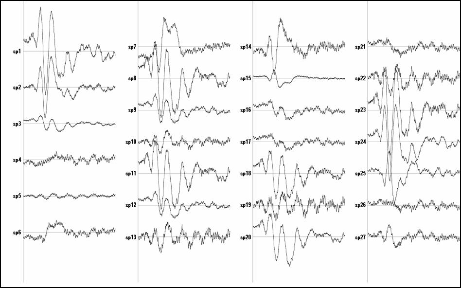
Figure 1:
Temporal activity estimated for the ACC
voxels.
Figure 1 shows the ELECTRA estimated traces for some voxels at the Anterior Cingulated Area (ACC) and Figure 2 for voxels at the primary visual area (V1). The selection of the voxels indexes was done using ACC defined as Brodmann area 32 and V1 defined as BA 17. Only a few voxels (27 out of 60 for ACC) are shown to illustrate the point. It is easy to see that some voxels show two positives and one negative peak (e.g., 1,2,23,24) while others mainly capture the noise (sp.4). Even others (e.g., sp 14) show the first component but the latest positive component is much slower (less sharp).
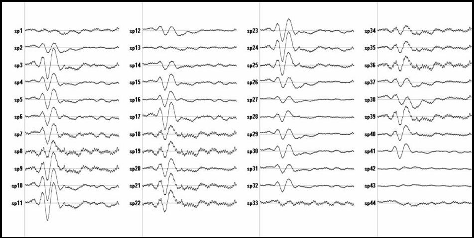
Figure 2: Primary visual cortex
2) The voxels selected when doing feature selection using ELECTRA are not neuro-physiologically interpretable while those obtained from the minimum norm (CDD) are. Is that true?
According to the neuroscience literature the selection of voxels proposed by ELECTRA is more distributed and therefore compatible with intracranial recording results on ERN. On the other hand the CCD selection misses the ACC and proposes the motor cingulate.In fact, according to the neuroscience literature the selection of voxels proposed by the CCD is not neurophysiologically interpretable. The image presented in Uldry et al. shows a localization covering something that looks like thalamus/white matter rather than Anterior Cingulate Cortex. A correct localization of the part of the ACC expected to participate in this task should be much more anterior and less buried. For instances, there is a famous study on a patient with ACC lesion and ER negativity showing a decrease of the Error negativity after anterior cingulated lession. Also diminished was his ability (and/or motivation) to correct erroneous responses.
3) Finally in the IDIAP report there is a sort of attempt to compare three different inverse solutions for the same data. This part is simply catastrophic from the methodological point of view. The most striking errors of this "comparison" are:
a) The three solutions use three absolutely different head models and solution points distribution. This is actually comparing pears and apples. Comparing sLORETA in a model with around 2000 points with CCD in a cortical model with the 4024 solutions point model of ELECTRA is simply inadmissible.
b) They compare a solution with a very high regularization parameter with solutions computed with nearly no regularization. Obviously, it is not the same a solution aimed at single trial data than a solution aimed at average data.
c) Using linear inverse solutions is unfortunately a little bit more tricky than multiplying a matrix by the data after transforming then to some reference. It implies many different steps violated in this study such as selection of the adequate regularization parameter and the source model.
d) Besides the fact that CCD uses an approximate source model neglecting the (obviously present!) deep sources, it is known to produce source distributions strikingly similar to the EEG surface maps. Regarding the use of the CCD, it has been established in Deliverable 3.1 (first year of MAIA project) that the CCD has no advantages with respect to a simple Spline Laplacian of the EEG surface data during hand or feet movement imagination in 3 subjects (figure 11). In fact, the best result, were obtained for a simple surface Laplacian estimator. On that basis the surface laplacian must be preferred far before the CCD.
e) Since the transformation to compute the CCD from the EEG was not available on the MAIA web site (where was our transformation matrix) it was not possible to evaluate it, however it is rather clear from the theory that the time courses provided by the CCD will resemble much more between them than for a real 3D head model as used in ELECTRA.
Disclaimer
This site is not a FORUM. Nevertheless, it is inspired on the principles of the IEEE code of ethics and thus is supposed to show reliable information avoiding all kind of fallacies (e.g. “ad hominem” ). For that reason, if you can proof that the information provided here is inexact we will remove it and it will be re inserted only once it is correctly re- stated. Error and/or omissions on the topics described here are not intentional.
Back to TOP |
|
 |
|
 |